Not all tunnels are born equal; some can be your tomb. Not all vaccines are born equal; some can revive the epidemic. Not all software are born equal; some can cause air crashes. In this post, I will show you how a meticulous programmer can uncover the truth that even Richard Sutton has missed.

Richard Sutton is a distinguished research scientist at DeepMind and a professor of computing science at the University of Alberta. He is considered one of the founding fathers of modern computational reinforcement learning.

Sutton is also an excellent educator. His textbook Reinforcement Learning: An Introduction, fluid and having a good rythme, is one of my all time favorites.

Recently, I am reading this book for the second time, and I found a thing that Sutton has neglected about the greedy algorithm (described in Chapter 2) for the bandit problem. In this post, I will present my discovery and provide extensive evidence and reasoning to support it. After you finish reading this post, I hope you to realize the critical role rigorous programming can play.

This post is organized as follows. First, I will present the bandit problem and the greedy approach to crack the problem. Then, I will explain how Sutton’s “clever” computational device ended with misguiding him and led him to believe something false. Finally, I will compare my implementation with the others’ as well as provide extensive experiment results to support my findings. This discovery is original, just like all my other posts.

The bandit problem

The bandit problem is a classic one in reinforcement learning, and it is usually the first item taught. The bandit is actually a machine, which has a better-known name as the slot machine.

The machine shown above has only one arm, whereas the bandit machine in reinforcement learning has multiple arms, with each arm having a different reward distribution. For example, the following figure shows the reward distribution of a ten-armed bandit.

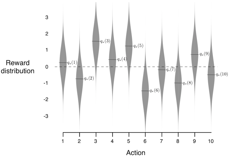
Obviously, the proprietor of the casino will not tell you the distribution. You have to find the optimal one yourself and find it as early as possible.

The $\varepsilon$-greedy algorithm

By the law of large number, the optimal arm is the one with the highest expectation. Therefore, the goal is to pull again and again the arms with high expectation. The higher, the better.

Also by the law of large number, the expectation of an arm can be estimated with the sample mean. That is, the accumulated reward on one arm divided by the total count of pulls on that arm gives an excellent estimation of the expectation.

Denote $q(a)$ as the expectation of the arm $a$ and $Q_t(a)$ as its estimation at time $t$. We have [ Q_t(a) := \frac{\sum_{i=1}^{t-1} R_i \cdot {1}_{A_i=a}}{\sum_{i=1}^{t-1} {1}_{A_i=a}}, ] where $R_i$ is the reward at time $i$ and $A_i$ is the arm pulled at time $i$.

The greedy algorithm consists of pulling the arm with currently the highest estimation. That is, [ A_t := \arg\max_a Q_t(a) ]

One problem with the greedy algorithm is that it is too rushy. If the optimal arm fails to behave well in its first pull, it will no longer be considered. (God knows how many girls missed their charming princes.)

Thus, Sutton advocates the $\varepsilon$-greedy algorithm, which has a probability of $\varepsilon$ to deviate from the current best arm and pick an arm in random. In this way, the algorithm explores other arms, and the charming prince optimal arm may get a second chance.

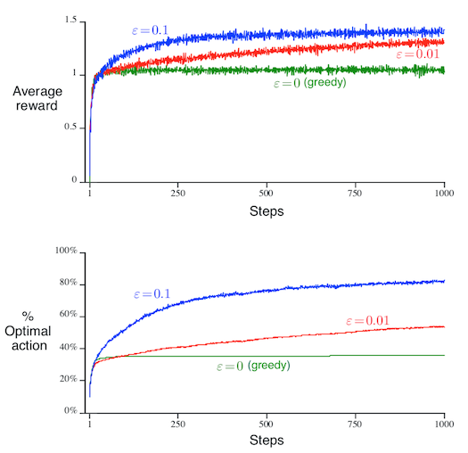
Sutton’s experiment shows that the $\varepsilon$-greedy algorithms outperform the (pure) greedy algorithm, in both the average reward and the percentage of optimal arm pulled.

Later in this post, I will show you that Sutton’s conclusion is wrong. But before that, let me first introduce you to Sutton’s “clever” computational device.

Sutton’s efficient update of the estimation

The expectation of the estimation can be, naively, calculated from the accumulated reward and the count. Sutton, being a genius, would certainly avoid we commoners’ path and do something smart instead. Indeed, he updated the estimation from the past one in a recurrent manner: [ Q_t = Q_{t-1} + (R_t - Q_{t-1}) / t. ] In this way, he saved the memory as well as accelerated the computation. Moreover, since the initial accumulated reward and count are both zero, the above formulation avoids the 0/0 error by manually setting the initial estimation.

Sutton picked zero for the initial estimation. He did not give the reason, but I can understand what he was thinking.

• Accumulated rewards start with zero, so it is natural to start the reward estimation with zero.
• The initial estimation serves as a prior just like in Bayesian statistics, so zero matches a zero-information prior just like the constant prior Bayesian statisticians would do.

The hidden parameter

Sutton launched the computation without a second thought, but let us analyze here the soundness of the above reasoning.

Q: Accumulated rewards start with zero, so it is natural to start the reward estimation with zero?

A: Both the accumulated reward and the count start with zero. Therefore, it is 0/0, which can be any number. Replacing an arbitrary number with zero does not sound right.

Q: Zero for the initial estimation matches a zero-information prior?

A: In Bayesian statistics, a constant prior does not give any privilege to any parameter value. However, it is true only for this parametrization. After a parameter transformation, a constant prior is no longer constant. Therefore, there is no real zero-information prior; every prior sneaks in some information. Similarly, assuming the initial estimation of expectation to be zero is just as informative as assuming it to be any other value.

In conclusion, the initial estimation is a parameter of the algorithm just like the parameter $\varepsilon$.

Sutton’s algorithm is one with two parameters instead of just one!

Tuning the initial estimation

All parameters can be tuned; so is the initial estimation. Here, I will give the experiment results generated with Zhang Shangtong’s code. I changed the initial estimation from 0 to 3 and -3.

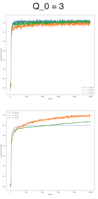
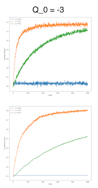
We can observe that the difference is huge by varying the initial estimation. For the value 3, the pure greedy algorithm works as well as the $\varepsilon$-greedy algorithms, if not better, in terms of average reward. For the value -3, the pure greedy algorithm just fails, whereas the $\varepsilon$-greedy algorithms adapt quite well.

This huge difference raises the question why the initial estimation plays such a critical role. To answer this question, it suffices to check the execution of the algorithm. In our experiment, the rewards are mainly located in $[-5, 5]$, so a value of 3 is a quite decent reward and a value of -3 is quite poor. An optimistic initial estimation encourages the algorithm to explore, to look for better reward in this nourishing world. A poor initial estimation reflects a pessimistic mindset, which refrains the algorithm from exploring.

Surprisingly, the initial estimation itself is also a parameter reflecting the explore-exploit tradeoff, just like the $\varepsilon$. Moreover, it plays an upper hand. In this regard, the parameter $\varepsilon$ is only secondary to the parameter initial estimation. The initial estimation explains the performance more than the $\varepsilon$ does. A good initial estimation waives the necessity of $\varepsilon$.

Remove the hidden parameter

It is difficult to evaluate an algorithm with two parameters. With the interference of the initial estimation, we can hardly judge the effect of $\varepsilon$ alone. To proceed, I propose to replace the subjective initial estimation with an objective one, namely by trying each arm once in the first place.

The following figure shows my experiment result. The legend items can be clicked to filter the curves. Although the pure greedy algorithm does not identify the optimal arm as often as the $\varepsilon$ versions, it is still the best in terms of average reward. The explanation is that it can often find the second best arm, whereas the $\varepsilon$ versions often waste their time in trying random (and bad) arms.

This result will not change even though the variance of the reward of each arm gets larger. The reason is that the motivation to find the absolute optimal arm is even weaker since chances play a more important role than choices do. The following figure shows the experiment result with a standard variation of 5.

The code to generate these plots can be found on my GitHub.

Conclusion

If the goal is to identify the optimal arm, then the $\varepsilon$-greedy versions win. If the goal is to gain high reward, then the pure greedy version is a safe bet.

Self-promotion time

This discovery would not be possible without my meticulous attitude toward programming. Just like I have always believed, rigorous and methodical programming can uncover truths and save the world.

In this regard, I might as well explain the advantages of my implementation over Zhang Shangtong’s.

• My implementation is truly object-oriented, whereas Shangtong’s uses an anti-pattern knowns as the God object.
• In my experiment, all algorithms are tested on a common set of 2000 bandits for fair comparison, whereas, in Shangtong’s experiment, each algorithm works on a different set of 2000 bandits.
• My implementation also provides an experiment where various algorithms work on the same bandit over and over instead of on 2000 independent bandits.
• My implementation allows the configuration of the standard variation of the reward.

For now, my repository is quite simple. I will probably add more items in the future depending on how soon I will find my next occupation. If you like my implementation, don’t hesitate to star and share it.

Update in 2021-08-09

• Sutton acknowledged, in his book, the role of the initial estimate only for the constant step size update, but not for the sample-average update. In addition, it is true that the sample-average update may not work well in nonstationary scenario (as Sutton mentioned in the book), but this disadvantage does not disqualify it for the stationary scenario.

• Sutton makes another mistake in Exercise 2.7, where the unbiased constant-step-size trick is presented. The idea is to start with a step size 1 and move toward a constant step size $\alpha$. Nevertheless, this trick cannot avoid the initial bias because the initial estimates are already in use even before they are overwritten by their respective first update. For instance, assuming the 1st arm updated, we need to decide the next arm to pull. We have to compare the reward we just received with the initial estimates of all other arms not yet pulled. Hence the initial bias. The following figure shows the experiment result.

• The above two mistakes are actually related. Sutton thought that, for both the sample-average update and the the unbiased constant-step-size trick, the initial estimates will be overwritten immediately after their respective first pull. Therefore, for him, the initial estimates do not have a role as in the constant step size case. However, these initial estimates are already in use before they are updated, and therefore they cannot be ignored.

Update in 2021-08-11

Sutton concluded the chapter with a parameter study (Figure 2.6 in his book). Here, I will do the same but with something more powerful.

Sutton noticed that it would be visually infeasible to present the temporal dimension with so many algorithms, so he presented the average reward across time instead, which is equivalent to the AUC (area under curve). Here, since we are on website, I can use animation to show the temporal dimension.

Reward across time

% of optimal pull across time

One thing of particular interest here is that all curves go up and down at the same rythme. This is because all algorithms work on the same bandit (with the same random number generator) in each simulation. A bad day for one algorithm is also a bad day for the others.

We can observe that the optimistic algorithm starts the fastest, and the gradient method starts slowly but later catches up. All algorithms can achieve good results asymptotically.