Many talk about data science and machine learning with enthusiasm, but few know about one of the most important building components behind them – convex optimization. Indeed, nowadays nearly every data science problem will first be transformed into an optimization problem and then solved by standard methods. Convex optimization, albeit basic, is the most important concept in optimization and the starting point of all understanding. If you are an aspiring data scientist, convex optimization is an unavoidable subject that you had better learn sooner than later.

This post will present several important inequalities in convex optimization, which are useful tools for proving the convergence of algorithms such as gradient descent. Unlike many books which just list the inequalities and the proofs and then call it a day, I will gently develop the intuition behind them. If you are someone who barely memorizes anything in the classic books of Stephen P. Boyd and of Yurii Nesterov after closing the books, this post is for you. After reading this post, you are expected to be able to understand the convergence analysis of most gradient-based algorithms.

The inequalities that I am going to prove and develop the intuition for are the following: [ \tfrac{\alpha}{2} \lVert x^* - x \rVert_2^2 \le f(x) - f(x^*) \le \tfrac{1}{2\alpha} \lVert \nabla f(x) \rVert_2^2 , ]

[ \tfrac{\beta}{2} \lVert x^* - x \rVert_2^2 \ge f(x) - f(x^*) \ge \tfrac{1}{2\beta} \lVert \nabla f(x) \rVert_2^2 , ]

where $f$ is an $\alpha$-strongly convex, $\beta$-smooth function, and $ x^* $ is the minimum point as usual. The term $ f(x) - f( x^* ) $ is called primal suboptimality and is the measure that we want to quantify in a convergence analysis.

Most of the above inequalities hold for both constrained and unconstrained optimization, and I will provide more clarification as well as a reference card later. In the following, I will use the $\alpha$-strongly convexity to prove the first pair of inequalities and $\beta$-smoothness to prove the second pair.

Table of contents

• $\alpha$-strongly convexity
• $\beta$-smoothness
• Usefulness of these inequalities
• Summary and further reading

$\alpha$-strongly convexity

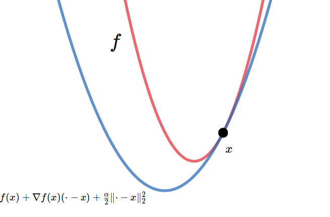
By definition, a function $f: \mathcal{D} \subset \mathbb{R}^n \rightarrow \mathbb{R}$ is $\alpha$-strongly convex if [ f(y) \ge f(x) + \nabla f(x) (y-x) + \tfrac{\alpha}{2} \lVert y-x \rVert_2^2 \quad \forall x, y \in \mathcal{D} . ]

This definition means that we can draw a parabola supporting the function curve at any point (Figure 1), and this parabola has a curvature characterized by the parameter $\alpha$. With this definition, we are going to both lower-bound and upper-bound the primal suboptimality $f(x)-f( x^* )$.

If you are talented, you will have discovered the “raw form” of $ f(x) - f( x^* ) $ inside the definition. That is, by alternately making $x$ and $y$ equal to $ x^* $, we will have $ f(y) - f( x^* ) \ge \ldots $ and $ f( x^* ) - f(x) \le \ldots $, which in turn give the lower and upper bounds. All we have to do is to transform the remaining terms into what we would like. In the following, I will first develop the intuition and then the math.

Lower bound

The lower bound to prove indicates that the primal suboptimality is bounded by the distance to the optimum point. To understand how it is possible, let us draw the supporting parabola at the optimum point (Figure 2). We easily see that the primal suboptimality for any point $x$ is at least $\tfrac{\alpha}{2} \lVert x-x^* \rVert_2^2$.

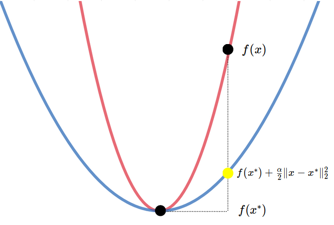
Mathematically, inside the definition, taking $ x=x^* $ gives us [ f(y) - f( x^* ) \ge \nabla f( x^* ) ( y-x^* ) + \tfrac{\alpha}{2} \lVert y-x^* \rVert_2^2 \quad \forall y \in \mathcal{D} . ]

In unconstrained optimization (i.e., $\mathcal{D}=\mathbb{R}^n$), the gradient at the minimum point is zero (i.e., $\nabla f( x^* ) = 0$). In constrained optimization (i.e., $\mathcal{D} \subsetneq \mathbb{R}^n$), we have the Karush-Kuhn-Tucker (KKT) condition, which implies that $ \nabla f( x^* ) ( y-x^* ) \ge 0, \forall y \in \mathcal{D}$. In both cases, we have [ f(y) - f( x^* ) \ge \tfrac{\alpha}{2} \lVert y-x^* \rVert_2^2 \quad \forall y \in \mathcal{D} . ]

Upper bound

The upper bound says the primal suboptimality is upper bounded by the current gradient. This upper bound is useful, for it is a potential termination condition for the optimization algorithm.

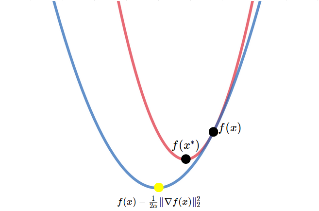
To understand how it is possible, let us draw the supporting parabola at any point $x$ (Figure 3). Since it is a parabola, any junior middle school student can calculate its minimum, which is $ f(x) - \tfrac{1}{2\alpha} \lVert \nabla f(x) \rVert_2^2 $. This minimum is, of course, lower than any point in $f$ (including the minimum of $f$).

Mathematically, although we would like to take $ y=x^* $ as in the lower bound case, we cannot use this approach here. Otherwise, we will have to handle the incoming $\nabla f(x)(x^* -x)$ term, which looks hopeless. Therefore, we will use a more careful approach, and this approach will also be used to prove the upper bound for $\beta$-smooth functions.

More specifically, we consider the right-hand side of the definition as a function of $y$ (or equivalently, as a functional of $x$) and minimize it on $y$. Since it is a parabola in terms of $y$, its minimum is given as $ f(x) - \tfrac{1}{2\alpha} \lVert \nabla f(x) \rVert_2^2 $. After this transition, the right-hand side is a function of $x$ solely and does not depend on $y$, which allows us to take minimum on the left-hand side with regard to $y$, which in turn gives $f( x^* )$. Hence, we have [ f( x^* ) \ge f(x) - \tfrac{1}{2\alpha} \lVert \nabla f(x) \rVert_2^2 . ]

By simply reorganizing the terms, we get the upper bound.

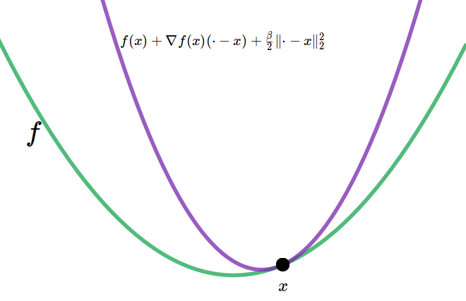
$\beta$-smoothness

By definition, a function $f: \mathcal{D} \subset \mathbb{R}^n \rightarrow \mathbb{R}$ is $\beta$-smooth if [ f(y) \le f(x) + \nabla f(x) (y-x) + \tfrac{\beta}{2} \lVert y-x \rVert_2^2 \quad \forall x, y \in \mathcal{D} . ] It gives the opposite direction to the one in the definition of $\alpha$-strongly convexity. This definition means that we can draw a parabola covering the function curve at any point (Figure 4), and this parabola has a curvature characterized by the parameter $\beta$. With this definition, we are going to both upper-bound and lower-bound the primal suboptimality $ f(x) - f( x^* ) $. As in the $\alpha$-strongly convexity, I first develop the intuition and then the proof.

Upper bound

The upper bound to prove indicates that the primal suboptimality is bounded by the distance to the optimum point. To understand how it is possible, let us draw the covering parabola at the optimum point (Figure 5). We easily see that the primal suboptimality for any point $x$ is at most $\tfrac{\beta}{2} \lVert x-x^* \rVert_2^2$.

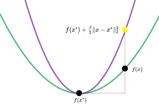
Mathematically, inside the definition, taking $ x=x^* $ gives us [ f(y) - f( x^* ) \le \nabla f( x^* ) ( y-x^* ) + \tfrac{\beta}{2} \lVert y-x^* \rVert_2^2 \quad \forall y \in \mathcal{D} . ]

In unconstrained optimization (i.e., $\mathcal{D}=\mathbb{R}^n$), the gradient at the minimum point is zero (i.e., $\nabla f( x^* ) = 0$), which nullifies the first term on the right-hand side. In constrained optimization (i.e., $\mathcal{D} \subsetneq \mathbb{R}^n$), unlike in the $\alpha$-strongly convexity, the KKT condition will not help, except if the minimum point is in the interior of $\mathcal{D}$, which nullifies the gradient. Therefore, only in unconstrained optimization and some cases in constrained optimization, we have the upper bound [ f(y) - f( x^* ) \le \tfrac{\beta}{2} \lVert y-x^* \rVert_2^2 \quad \forall y \in \mathcal{D} . ]

Lower bound

The lower bound says the primal suboptimality is lower bounded by the current gradient. To understand how it is possible, let us draw the covering parabola at any point $x$ (Figure 6). Since it is a parabola, any junior middle school student can calculate its minimum, which is $ f(x) - \tfrac{1}{2\beta} \lVert \nabla f(x) \rVert_2^2 $. This minimum is, of course, higher than the minimum of $f$.

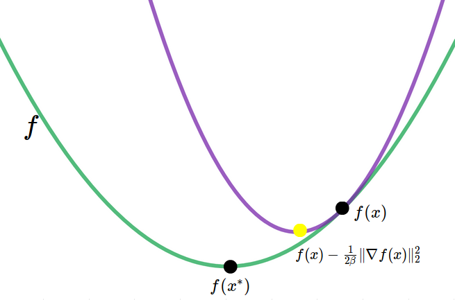
Mathematically, we shall use a similar technique as in $\alpha$-strongly convexity. More specifically, we consider the right-hand side of the definition as a function of $y$ (or equivalently, as a functional of $x$) and minimize it on $y$. Since it is a parabola in terms of $y$, its minimum is given as $ f(x) - \tfrac{1}{2\beta} \lVert \nabla f(x) \rVert_2^2 $. After this transition, the right-hand side is a function of $x$ solely and does not depend on $y$, which allows us to take minimum on the left-hand side with regard to $y$, which in turn gives $f( x^* )$. Hence, we have [ f( x^* ) \le f(x) - \tfrac{1}{2\beta} \lVert \nabla f(x) \rVert_2^2 . ]

By simply reorganizing the terms, we get the lower bound.

Usefulness of these inequalities

One may wonder about these specific forms of inequalities and want to know why they are useful. Judging from the fact that the definitions of $\alpha$-strongly convexity and of $\beta$-smoothness already give the upper and lower bounds, these particular forms of inequalities seem redundant.

The fact is that those “raw” forms of inequalities are hard to use, for they contain two different terms: $\nabla f(x)$ and $( x-x^* )$. On the other hand, the proven inequalities are concise, for they contain only one term: either $\nabla f(x)$ or $( x-x^* )$. This simplicity will enable, in the convergence analysis, a trick known as recurrence.

Let us see this, for instance, through the analysis of gradient descent for unconstrained optimization, whose iteration is given by [ x_{t+1} := x_t - \tfrac{1}{\beta} \nabla f(x_t). ] Denoting $h_t:=f(x_t) - f( x^* )$ as the primal suboptimality at $t$-th iteration, we get \[ \begin{align} h_{t+1} - h_t & = f(x_{t+1}) - f(x_t) \newline & \le \nabla f(x_t) (x_{t+1} - x_t) + \tfrac{\beta}{2} \lVert x_{t+1} - x_t \rVert_2^2 \qquad \beta\text{-smoothness} \newline & = - \tfrac{1}{\beta} \lVert \nabla f(x_t) \rVert_2^2 + \tfrac{1}{2\beta} \lVert \nabla f(x_t) \rVert_2^2 \qquad \text{algorithm} \newline & = - \tfrac{1}{2\beta} \lVert \nabla f(x_t) \rVert_2^2 , \end{align} \] which implies that the primal suboptimality is reduced by a certain quantity characterized by the norm of the gradient.

Remembering that the norm of the gradient is lower-bounded by the primal suboptimality (using the 2nd proven inequality reversely), we further have [ h_{t+1} - h_t \le - \tfrac{1}{2\beta} \lVert \nabla f(x_t) \rVert_2^2 \le - \tfrac{\alpha}{\beta} h_t, ] which gives us a dynamic concerning $h_t$: [ h_{t+1} \le h_t (1-\tfrac{\alpha}{\beta}), ] from where [ h_{t+1} \le h_1 (1-\tfrac{\alpha}{\beta})^t . ] We proved, thereby, the linear convergence of gradient descent for $\alpha$-strongly convex, $\beta$-smooth functions.

Summary and further reading

In this post, I proved four inequalities. Their applicability can be summarized in the following table.

$f(x)-f(x^*)$	$\alpha$-strongly convex	$\beta$-smooth	Extra conditions
$\ge \tfrac{\alpha}{2} \lVert x^* - x \rVert_2^2$	Y
$\le \tfrac{1}{2\alpha} \lVert \nabla f(x) \rVert_2^2$	Y
$\le \tfrac{\beta}{2} \lVert x^* - x \rVert_2^2$		Y	$x^*\in\mathring{\mathcal{D}}$
$\ge \tfrac{1}{2\beta} \lVert \nabla f(x) \rVert_2^2 $		Y

You can use these inequalities in various directions: they give bounds not only for the primal suboptimality but also for the distance to the optimum point and the norm of the gradient. We have already seen, in the analysis of the gradient descent, how to use the 2nd inequality to lower-bound the norm of the gradient. Used correctly, they will be powerful tools during the convergence analysis for your own algorithms.

This post must stop here. If you want to learn more about convex optimization, you can proceed with functions that are not strongly convex or that smooth. You can also study the stochastic gradient descent, proximal methods and Frank-Wolfe methods. Besides, you can also study online convex optimization and non-convex optimization. There is plenty to study in this domain, and I am sure you will not get bored.